Plotting Survival Curves after fitting Cox Proportional Hazards Models

R Code

Introduction

I got a question from a clinician asking if Cox Proportional Hazards (PH) models do not estimate baseline hazards, how did we plot survival curves after fitting a Cox model?

Cox PH models have this love-hate relationship with baseline hazards. The advantage of Cox models is that we can estimate hazard ratios without specifying the baseline hazard function. The disadvantage is that we do not estimate the baseline hazard function. (Basically its advantage = disadvantage. Haha!)

When we need to plot survival curves after fitting a Cox model, we don’t directly estimate the baseline hazard during model fitting. Instead, we estimate it afterward using methods like the Breslow estimator (aka, the Nelson-Aalen estimator). This post will explain how we can obtain baseline hazards and plot survival curves after fitting a Cox PH model.

The Cox Proportional Hazards Model

The Cox PH model is specified as:

$$h(t|\mathbf{X})=h_0(t)\exp (\mathbf{X}\hat{\beta })$$

Where:

• $h(t|\mathbf{X})$ is the hazard at time $t$ for an individual with covariates $\mathbf{X}$
• $h_0(t)$ is the baseline hazard (when all covariates are 0)
• $\beta$ are the estimated coefficients

The model estimation uses partial likelihood to estimate $\beta$ without specifying $h_0(t)$, which is what makes Cox regression semi-parametric.

Estimating the Baseline Hazard

After fitting the Cox model, the Breslow estimator is commonly used to estimate the baseline cumulative hazard function:

$${\hat{H}}_0(t)=\sum _{j=1}^k\frac{d_j}{\sum _{i\in R(t_j)}\exp (\mathbf{X}\hat{\beta })}$$

Where:

• $d_j$ is the number of events at the $j$th ordered event time, $t_j$
• $R(t_j)$ is the risk set at time $t_j$ (individuals still at risk)
• $\exp (\mathbf{X}\hat{\beta })$ is the risk score for individual $i$.

The baseline survival function is then calculated as:

$${\hat{S}}_0(t)=\exp (-{\hat{H}}_0(t))$$

Covariate Patterns for Prediction

When predicting survival curves from a Cox model, we need to decide what covariate values to use:

1. Average covariates: The default in survival::survfit() when newdata argument is not specified. This does not always make sense, especially for categorical variables (Nieto and Coresh, 1996). For example, the average value of sex == 1 (male) and sex == 0 (female) is 0.5, which is not meaningful on the individual level.
2. Baseline values: Setting covariates to specific reference values (e.g., all zeros).
3. Conditional predictions: Conditional on certain characteristics (e.g., age = 50 and sex = “male”).
4. Marginal survival curves: Predicting survival for each individual in the dataset and then averaging the survival probabilities at each time point.
5. Standardized survival curves: Predicting survival for a standard population, either to an internal or external population(e.g., age-standardized)(Syriopoulou 2022).

The predicted survival function for a specific covariate pattern $\mathbf{X}$ is:

$$\hat{S}(t|\mathbf{X})=[{\hat{S}}_0(t){]}^{\exp (\mathbf{X}\hat{\beta })}=\exp (-{\hat{H}}_0(t)\cdot \exp (\mathbf{X}\hat{\beta }))$$

Caution

It’s common to read in Epi articles that authors present adjusted survival curves after fitting a Cox PH model without specifying how they set the covariates. Sometimes they use average covariates without noticing that some of their covariates are categorical.

Once, someone told me that since it’s Cox model, it does not matter what covariates you set because the hazard ratios are constant over time. This is incorrect. The hazard ratios are indeed constant over time (so it does not matter what covariates one predict from), but the survival probabilities depend on the covariate values you choose. Simply look at the equation above: the survival function depends on $\exp (\mathbf{X}\hat{\beta })$, which varies with different covariate patterns.

Practical Example in R

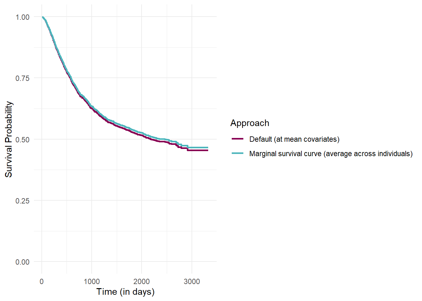
Let’s demonstrate the difference between 1. Average covariates and 4. Marginal survival curves using with the colon dataset from the survival package:

# Load necessary libraries
library(survival)
library(ggplot2)
library(dplyr)

# Load the colon cancer dataset from the survival package
colon <- na.omit(survival::colon)

# Fit the Cox model
coxph_model <- coxph(Surv(time, status) ~ age + sex, data = colon)

# Approach 1: Predict survival curve at the mean values of covariates ---
# This is the default behavior when newdata is not specified.
# survfit() creates a curve for a single hypothetical person with mean age and mean sex.
fit1 <- survfit(coxph_model)

# Extract the data into a data frame for plotting
dffit1 <- data.frame(time = fit1$time,
                     surv_prob = fit1$surv,
                     method = "Default (at mean covariates)")

# Approach 2: Predict for each individual and then average the curves
# By passing the original data to newdata, we get a survival curve for each person.
fit2 <- survfit(coxph_model, newdata = colon)

# The result 'fit_individual$surv' is a matrix where each column is a person's
# predicted survival curve. We calculate the row-wise mean to get the
# average survival probability at each time point.
avg_surv_prob <- rowMeans(fit2$surv)

# Create a data frame for the marginal survival curve
dffit2 <- data.frame(
  time = fit2$time,
  surv_prob = avg_surv_prob,
  method = "Marginal survival curve (average across individuals)"
)

# Plot
# Combine the two data frames into one for easy plotting with ggplot2
df <- bind_rows(dffit1, dffit2)

# Plot both curves on the same plot
ggplot(df, aes(x = time, y = surv_prob, color = method)) +
  geom_step(linewidth = 1) + # Use geom_step for survival curves
  labs(
    x = "Time (in days)",
    y = "Survival Probability",
    color = "Approach"
  ) +
  theme_minimal() +
  scale_color_manual(values = c("Default (at mean covariates)" = "#870052", 
                                "Marginal survival curve (average across individuals)" = "#4DB5BC")) +
  coord_cartesian(ylim = c(0, 1))

From the example above, we can see that the two approaches yield different survival curves. Though we use the same Cox model (have the same coefficients), the choice of covariate patterns for prediction matters. They look similar, but the interpretations are totally different.

The default method (using mean covariates) may not accurately represent the study population’s survival experience, as it predicts from sex = 0.5 and age = mean(age). The marginal survival curve, which averages individual predictions, shows the average survival probabilities across the cohort. In this example, I recommend using the marginal survival curve for a more representative estimate of survival in the study population.

Now when people say they’ve adjusted survival curves after fitting Cox models, one should check how they set the covariates for prediction!

References

1. Nieto and Coresh. Adjusting Survival Curves for Confounders: A Review and a New Method. American Journal of Epidemiology, 1996.
2. Collett. Modelling Survival Data in Medical Research. 4ed. 2023.
3. Syriopoulou et al. Standardised survival probabilities: a useful and informative tool for reporting regression models for survival data. British Journal of Cancer. 2022. 127:1808–1815; https://doi.org/10.1038/s41416-022-01949-6.