Code
#### Load necessary packages ####

library(survival)
library(dplyr)
library(ggplot2)
library(broom)
library(tidyr)
library(gridExtra)
library(knitr)Following my previous post on Estimating survival when individual-participant data can’t be pooled: potential solutions, one of the solutions was to approximate the Cox model with a Poisson generalised linear model (GLM) (see the post on Replicating a Cox Model with Poisson Regression in R).
This post aims to go through a simulation study in R to demonstrate how this works and show just how accurate the approximation can be in such case.
“Is there a difference in survival for cancer patients who undergo fertility preservation compared to those who do not, after adjusting for potential confounders?”
We’ll simulate data for three different countries (A, B, and C), where patient characteristics and treatment patterns differ, to see how the models handle confounding.
First, let’s load the R packages we’ll need for data manipulation, modeling, and plotting.
#### Load necessary packages ####
library(survival)
library(dplyr)
library(ggplot2)
library(broom)
library(tidyr)
library(gridExtra)
library(knitr)I start by creating a dataset of 3,000 patients, randomly assigned to one of three countries (A, B, or C). I’ll introduce confounding to emulate the real-world scenario. For example, Country C will have an older population with a poorer prognosis, while Country B will have a younger population with a better prognosis. Also, I’ll make fertility preservation more likely among those getting chemotherapy.
#### Simulation Process ####
# Set seed
set.seed(13579)

#### Step 1: Simulate covariates to create confounding ####

# Create the data frame with country assignments
n <- 3000
simdata <- data.frame(country = sample(c("A", "B", "C"),
                                       n, replace = TRUE, prob = c(1/3, 1/3, 1/3)))

# Add covariates
covariates <- c("agegrp", "fp", "birthplace_europe", "education", "parity",
                "yeardx", "lymphnode", "tumorsize", "chemo")
simdata[, covariates] <- NA

# Get indices for each country to create different covariate distributions
idx_A <- which(simdata$country == "A")
idx_B <- which(simdata$country == "B")
idx_C <- which(simdata$country == "C")
n_A <- length(idx_A)
n_B <- length(idx_B)
n_C <- length(idx_C)

# Make Country A older than B/younger than C.
# Make Country B younger.
# Make Country C older.

# agegrp (1=young, 2=mid, 3=old)
simdata$agegrp[idx_A] <- sample(1:3, n_A, replace = TRUE, prob = c(0.4, 0.4, 0.2)) # A: Middle population
simdata$agegrp[idx_B] <- sample(1:3, n_B, replace = TRUE, prob = c(0.6, 0.3, 0.1)) # B: Younger population
simdata$agegrp[idx_C] <- sample(1:3, n_C, replace = TRUE, prob = c(0.1, 0.3, 0.6)) # C: Older population

# Make fertility preservation more likely among those getting chemo
# Make fp=1 with more chemo
# Make fp=0 with less chemo

# First assign chemotherapy status
simdata$chemo <- sample(0:1, n, replace = TRUE, prob = c(0.2, 0.8))

# Then assign fertility preservation status based on chemotherapy status
# For patients with chemo, higher probability of fertility preservation
simdata$fp <- rep(NA, n)
# For those not receiving chemo
simdata$fp[simdata$chemo == 0] <- sample(0:1, sum(simdata$chemo == 0),
                                         replace = TRUE, prob = c(0.8, 0.2))
# For those receiving chemo - higher chance of fertility preservation
simdata$fp[simdata$chemo == 1] <- sample(0:1, sum(simdata$chemo == 1),
                                         replace = TRUE, prob = c(0.4, 0.6))
# Simply a two-by-two to see whether the results are generated correctly
table(simdata$chemo, simdata$fp)
       0    1
  0  473  106
1 959 1462# Simulate other covariates uniformly
# Just for illustration
simdata$birthplace_europe <- sample(0:1, n, replace = TRUE)
simdata$education <- sample(1:3, n, replace = TRUE)
simdata$parity <- sample(0:2, n, replace = TRUE)
simdata$yeardx <- sample(0:1, n, replace = TRUE)
simdata$lymphnode <- sample(1:3, n, replace = TRUE)
simdata$tumorsize <- sample(0:3, n, replace = TRUE)
# Convert all covariates to factors for modeling
simdata[covariates] <- lapply(simdata[covariates], function(x) as.factor(as.character(x)))Now I’ll generate their survival times. We do this by defining a “true” model where we know the exact HRs for key variables. For instance, we’ll set the true HR for receiving chemotherapy to 5.0, a very strong effect. The effect of fertility preservation (fp) is set to be very small (HR = 1.05).
We then use these true HRs and a Weibull distribution to generate a unique survival time for each patient based on their covariate patterns. Finally, we censor everyone’s follow-up at 10 years.
# Define regression coefficients (log-hazard ratios) for the TRUE estimates
beta_agegrp3 <- log(2)    # HR=2.0 for agegrp 3 vs 1
beta_agegrp2 <- log(1.5)  # HR=1.5 for agegrp 2 vs 1
beta_chemo1  <- log(5)    # HR=5.0 for chemo vs no chemo
beta_fp1     <- log(1.2) # HR=1.05 for fp vs no fp

# Create the linear predictor from the covariates
lp <- ifelse(simdata$agegrp == 2, beta_agegrp2, 0) +
  ifelse(simdata$agegrp == 3, beta_agegrp3, 0) +
  (as.numeric(simdata$chemo) - 1) * beta_chemo1 +
  (as.numeric(simdata$fp) - 1) * beta_fp1

# Use a single baseline hazard for all individuals (Weibull distribution)
# with the proportional hazards assumption.
weibull_shape <- 1.2
weibull_scale <- 80

# Generate true survival times using the inversion method
# Now every individual has survival time according to their linear predictors
U <- runif(n) # Uniform random variables
time_true <- (-log(U) / ( (1/weibull_scale^weibull_shape) * exp(lp) ) )^(1/weibull_shape)

# Apply right-censoring at 10 years
time_censor <- 10
simdata$status <- ifelse(time_true > time_censor, 0, 1)
simdata$time <- pmin(time_true, time_censor)Now that we have our simulated dataset, let’s fit the Cox proportional hazards models. We’ll fit both unadjusted and adjusted models using the individual-level data. Theses results will serve as the TRUE estimates we aim to obtain afterwards by fitting a glm.
# Unadjusted Cox model
coxmod1 <- coxph(Surv(time, status) ~ fp , data = simdata)

# Adjusted Cox model
coxmod2 <- coxph(Surv(time, status) ~  fp + country + agegrp +
                   birthplace_europe + education +
                   parity + yeardx + lymphnode + tumorsize + chemo,
data = simdata)This part is what the site statistician/data handler should do to report aggregate-level data. First, we need to transform the data from an individual-level format to an aggregate-level data with person-time and event counts for each combination of covariates and time intervals. Last, the aggregated data will be sent to one place and used to fit a Poisson GLM to estimate hazard ratios.
Totally there are three steps: Steps A & B are done by the site statistician/data handler to create the aggregate dataset. Steps C is done by the analyst who receives the aggregate dataset.
status) and the total person-time (pt).offset(log(pt)). This tells the model that we are modeling the rate of events (events per person-time), which is exactly what a hazard rate is. We also include the time interval (fu) as a factor to allow the baseline hazard to vary over time, which is analogous to the non-parametric baseline hazard in a Cox model.# Step A & B are done by the site statistician/data handler to create the aggregate dataset.
# START HERE
# Create person-time data
max_time <- floor(max(simdata$time))
cut_points <- seq(0, max_time, by = 1)
# Split by country
list_by_country <- split(simdata, simdata$country)
# Process each country's data
df_list <- lapply(list_by_country, function(country_df) {
df_splityr <- survSplit(Surv(time, status) ~ ., data = country_df,
cut = cut_points, end = "time", start = "start",
event = "status")
df_splityr2 <- transform(df_splityr,
pt = time - start,
fu = as.factor(start))
df_splityr2 |>
group_by(fu, country, agegrp, fp, birthplace_europe, education,
parity, yeardx, lymphnode, tumorsize, chemo) |>
summarise(pt = sum(pt), status = sum(status), .groups = 'drop')
})
# END HERE# Step C is done by the analyst who receives the aggregate dataset.
# Then the main analyst combines the datasets from each country
# Combine into one aggregate dataset
simdata_ABC <- dplyr::bind_rows(df_list)
# Unadjusted GLM
glm1 <- glm(status ~ fu + fp + offset(log(pt)),
family = poisson, data = simdata_ABC)
# Adjusted GLM
glm2 <- glm(status ~ fu + country + agegrp + fp + birthplace_europe + education +
parity + yeardx + lymphnode + tumorsize + chemo + offset(log(pt)),
family = poisson, data = simdata_ABC)Let’s plot the survival curves from both the Cox models (using individual data) and the Poisson GLMs (using aggregated data) side-by-side.
#### Step 5: Plots ####

# Ensure factor levels are consistent
simdata$country <- factor(as.character(simdata$country), levels = c("A", "B", "C"))
simdata_ABC$country <- factor(as.character(simdata_ABC$country), levels = c("A", "B", "C"))
simdata$fp <- factor(as.character(simdata$fp), levels = c("0", "1"))
simdata_ABC$fp <- factor(as.character(simdata_ABC$fp), levels = c("0", "1"))

# Create average profile for predictions
avg_profile <- data.frame(
  country = factor("A", levels = levels(simdata_ABC$country)), # Average profile for country A
  agegrp = factor("1", levels = levels(simdata_ABC$agegrp)),
  birthplace_europe = factor("0", levels = levels(simdata_ABC$birthplace_europe)),
  education = factor("2", levels = levels(simdata_ABC$education)),
  parity = factor("1", levels = levels(simdata_ABC$parity)),
  yeardx = factor("0", levels = levels(simdata_ABC$yeardx)),
  lymphnode = factor("2", levels = levels(simdata_ABC$lymphnode)),
  tumorsize = factor("1", levels = levels(simdata_ABC$tumorsize)),
  chemo = factor("0", levels = levels(simdata_ABC$chemo))
)

# --- Cox Model 1 (Unadjusted) ---
cox1_curves_list <- lapply(c("0", "1"), function(fp_val) {
  newdata_temp <- data.frame(fp = factor(fp_val, levels = c("0", "1")))
  sf <- survfit(coxmod1, newdata = newdata_temp)
  df <- tidy(sf)
  df$fp <- fp_val
  return(df)
})
cox1_curves <- bind_rows(cox1_curves_list)

# --- Cox Model 2 (Adjusted) ---
cox2_curves_list <- lapply(c("0", "1"), function(fp_val) {
  newdata_temp <- avg_profile
  newdata_temp$fp <- factor(fp_val, levels = c("0", "1"))
  sf <- survfit(coxmod2, newdata = newdata_temp)
  df <- tidy(sf)
  df$fp <- fp_val
  return(df)
})
cox2_curves <- bind_rows(cox2_curves_list)

# Combine Cox data for plotting
plot_data_cox1 <- cox1_curves %>% arrange(fp, time)
plot_data_cox2 <- cox2_curves %>% arrange(fp, time)

# --- GLM Models: generate newdata for predictions ---
fu_levels <- sort(unique(as.numeric(as.character(simdata_ABC$fu))))

# Create newdata for GLM predictions
newdata_glm <- expand_grid(
  fp = factor(c("0", "1"), levels = levels(simdata_ABC$fp)),
  fu = fu_levels
) %>%
  mutate(
    country = avg_profile$country[1],
    agegrp = avg_profile$agegrp[1],
    birthplace_europe = avg_profile$birthplace_europe[1],
    education = avg_profile$education[1],
    parity = avg_profile$parity[1],
    yeardx = avg_profile$yeardx[1],
    lymphnode = avg_profile$lymphnode[1],
    tumorsize = avg_profile$tumorsize[1],
    chemo = avg_profile$chemo[1],
    pt = 1,
    fu = factor(fu, levels = as.character(fu_levels))
  )

# Function to calculate survival from GLM predictions
calculate_glm_surv <- function(newdata, predictions, fp_col = "fp") {
  df <- newdata %>%
    mutate(
      pred = predictions,
      hazard_rate = pred / pt,
      time = as.numeric(as.character(fu))
    )

  df <- df %>%
    arrange(fp, time) %>%
    group_by(fp) %>%
    mutate(survival = cumprod(exp(-hazard_rate))) %>%
    ungroup() %>%
    select(fp, time, survival)

  # Add baseline (time = 0, survival = 1)
  baseline <- df %>%
    distinct(fp) %>%
    mutate(time = 0, survival = 1)

  bind_rows(baseline, df) %>% arrange(fp, time)
}

# Generate GLM predictions and survival curves
pred_glm1 <- predict(glm1, newdata = newdata_glm, type = "response")
plot_data_glm1 <- calculate_glm_surv(newdata_glm, pred_glm1)

pred_glm2 <- predict(glm2, newdata = newdata_glm, type = "response")
plot_data_glm2 <- calculate_glm_surv(newdata_glm, pred_glm2)


#### Step 6: Create 2x2 Panel Plot for FP=0 vs FP=1 ####

color_palette_fp <- c("0" = "#0072B2", "1" = "#D55E00")
fp_labels <- c("0" = "No Fertility Preservation", "1" = "Fertility Preservation")

# Plot 1: Unadjusted Cox - FP
p1 <- ggplot(plot_data_cox1,
             aes(x = time, y = estimate, color = fp)) +
  geom_step(linewidth = 1.1) +
  scale_color_manual(values = color_palette_fp, labels = fp_labels) +
  labs(title = "Unadjusted Cox Model",
       x = "Time (Years)",
       y = "Survival Probability",
       color = "Treatment") +
  ylim(0, 1) +
  theme_minimal() +
  theme(legend.position = "none") +
  theme(plot.title = element_text(hjust = 0.5))


# Plot 2: Adjusted Cox - FP
p2 <- ggplot(plot_data_cox2,
             aes(x = time, y = estimate, color = fp)) +
  geom_step(linewidth = 1.1) +
  scale_color_manual(values = color_palette_fp, labels = fp_labels) +
  labs(title = "Adjusted Cox Model",
       x = "Time (Years)",
       y = "",
       color = "Treatment") +
  ylim(0, 1) +
  theme_minimal() +
  theme(legend.title = element_blank()) +
  guides(color = guide_legend(nrow = 1)) +
  theme(plot.title = element_text(hjust = 0.5))


# Plot 3: Unadjusted GLM - FP
p3 <- ggplot(plot_data_glm1,
             aes(x = time, y = survival, color = fp)) +
  geom_step(linewidth = 1.1) +
  scale_color_manual(values = color_palette_fp, labels = fp_labels) +
  labs(title = "Unadjusted Poisson GLM",
       x = "Time (Years)",
       y = "Survival Probability",
       color = "Treatment") +
  ylim(0, 1) +
  theme_minimal() +
  theme(legend.position = "none") +
  theme(plot.title = element_text(hjust = 0.5))

# Plot 4: Adjusted GLM - FP
p4 <- ggplot(plot_data_glm2,
             aes(x = time, y = survival, color = fp)) +
  geom_step(linewidth = 1.1) +
  scale_color_manual(values = color_palette_fp, labels = fp_labels) +
  labs(title = "Adjusted Poisson GLM",
       x = "Time (Years)",
       y = "",
       color = "Treatment") +
  ylim(0, 1) +
  theme_minimal() +
  theme(legend.position = "none") +
  theme(plot.title = element_text(hjust = 0.5))


# Extract legend function
get_legend <- function(plot) {
  tmp <- ggplot_gtable(ggplot_build(plot))
  leg <- which(sapply(tmp$grobs, function(x) x$name) == "guide-box")
  legend <- tmp$grobs[[leg]]
  return(legend)
}

# Extract the legend from p2
legend <- get_legend(p2)

# Remove legend from p2
p2 <- p2 + theme(legend.position = "none")

# Arrange 2x2 grid with legend at bottom
grid.arrange(
  arrangeGrob(p1, p2, p3, p4, ncol = 2),
  legend,
  nrow = 2,
  heights = c(10, 1)
)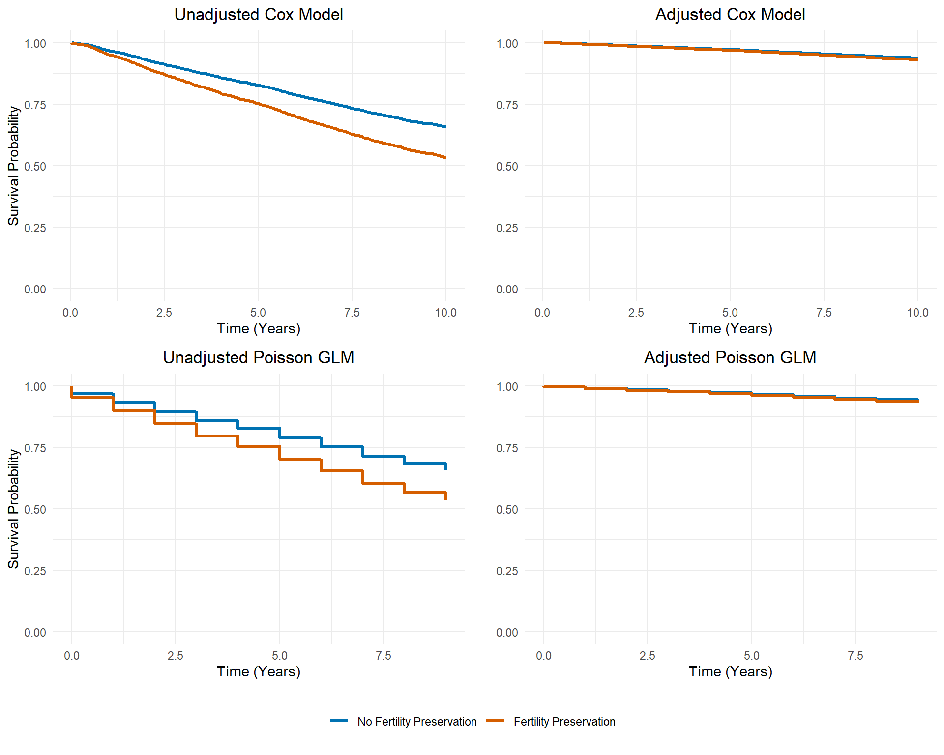
The Poisson GLMs (bottom row) approximate the survival curves from the Cox models (top row). Though we lost minor information by aggregating the data, the overall survival patterns were captured. Furthermore, adjustment of confounding can still be implemented using the aggregate data.
Now I’ll extract the coefficients from all our models, exponentiate them to get the HRs, and put them in a table for comparison.
# Extract coefficients and exponentiate
coef_cox1 <- tidy(coxmod1, exponentiate = TRUE) %>%
  select(term, estimate) %>%
  rename(cox_unadj = estimate)

coef_cox2 <- tidy(coxmod2, exponentiate = TRUE) %>%
  select(term, estimate) %>%
  rename(cox_adj = estimate)

coef_glm1 <- tidy(glm1, exponentiate = TRUE) %>%
  filter(!grepl("^fu", term), term != "(Intercept)") %>%
  select(term, estimate) %>%
  rename(glm_unadj = estimate)

coef_glm2 <- tidy(glm2, exponentiate = TRUE) %>%
  filter(!grepl("^fu", term), term != "(Intercept)") %>%
  select(term, estimate) %>%
  rename(glm_adj = estimate)

# Combine all coefficients
coef_table <- full_join(coef_cox1, coef_cox2, by = "term") %>%
  full_join(coef_glm1, by = "term") %>%
  full_join(coef_glm2, by = "term") %>%
  filter(!is.na(term)) %>%
  select(term, cox_unadj, glm_unadj, cox_adj, glm_adj)

# Print the table
print(kable(coef_table, digits = 4,
            caption = "Comparing HRs: Cox vs Poisson GLM"))
Table: Comparing HRs: Cox vs Poisson GLM

|term               | cox_unadj| glm_unadj| cox_adj| glm_adj|
|:------------------|---------:|---------:|-------:|-------:|
|fp1                |    1.4979|    1.4975|  1.1075|  1.1075|
|countryB           |        NA|        NA|  0.9970|  0.9969|
|countryC           |        NA|        NA|  0.9555|  0.9556|
|agegrp2            |        NA|        NA|  1.6433|  1.6426|
|agegrp3            |        NA|        NA|  2.1819|  2.1806|
|birthplace_europe1 |        NA|        NA|  1.0842|  1.0840|
|education2         |        NA|        NA|  0.9782|  0.9783|
|education3         |        NA|        NA|  0.9782|  0.9782|
|parity1            |        NA|        NA|  0.9725|  0.9724|
|parity2            |        NA|        NA|  0.9499|  0.9500|
|yeardx1            |        NA|        NA|  1.0136|  1.0133|
|lymphnode2         |        NA|        NA|  1.0843|  1.0840|
|lymphnode3         |        NA|        NA|  1.1152|  1.1148|
|tumorsize1         |        NA|        NA|  0.9942|  0.9941|
|tumorsize2         |        NA|        NA|  1.0641|  1.0638|
|tumorsize3         |        NA|        NA|  1.0266|  1.0264|
|chemo1             |        NA|        NA|  5.9553|  5.9496|
Look at the estimates for our main variable of interest, fp1 (fertility preservation), after adjusting for confounding. The Cox model estimates an HR of 1.1075, and the Poisson GLM estimates 1.1075. They are close!
The same holds true for the other covariates, including the strong confounder chemo1 and the agegrp effects. This demonstrates that the Poisson GLM can approximate the HRs from the Cox PH model.
By splitting the follow-up period into intervals and using the GLM, we can approximate estimate hazard ratios that are nearly close to those from a Cox model. This approach allows us to analyze survival data even when individual-level data cannot be shared across borders, while still adjusting for confounding factors.